NVIDIA Jetbot Gesture Recognition

The Jetbot is an open-source robot platform powered by the NVIDIA Jetson Nano. This project focuses on enabling the Jetbot to recognize gestures and respond with corresponding actions, combining cutting-edge machine learning and robotics techniques.

Project Overview

The goal of this project was to implement a scalable gesture recognition system that allows the Jetbot to classify specific hand gestures and execute predefined actions. Additional functionalities such as collision avoidance and object tracking were integrated for robust real-world operation. A detailed presentation can be found here.

Project Features

• Gestures Recognition: Classify specific gestures and trigger actions.
• Collision Avoidance: Detect and navigate around obstacles.
• Object Tracking: Identify and follow selected objects.
• General Logic: Integrate gesture recognition and collision avoidance into a cohesive control strategy.

Implementation Process

• Model optimization using ResNet to reduce size and retain accuracy.
• Obstacle avoidance using data augmentation and real-world testing.
• Utilized Docker to streamline deployment and system reproducibility.
• Initial tests with OpenCV were replaced with more accurate transfer learning approaches.

Key Functionalities

Collision Avoidance

Collision avoidance was achieved by training a ResNet-based model on a dataset of obstacles and clear paths. Data augmentation techniques such as flips, zooms, and contrast adjustments increased robustness, allowing the Jetbot to navigate safely in dynamic environments.

Gestures Recognition

The robot was trained to recognize gestures such as "Go Right" and "Go in Circles." When these gestures are detected, the Jetbot executes corresponding actions.

Go Right Gesture

Go Circles Gesture

TurtleBot Maze Solver

The TurtleBot is a ROS-based mobile robot. This project aimed to create a robust solution for navigating mazes using ROS2, laser distance sensors (LDS), odometry, and efficient navigation algorithms.

Project Overview

Figure 1: Initial 2x2 maze solving (left) and more advanced methods in 3x3 maze (right).

Setup Guide

This report provides a comprehensive walkthrough for setting up the environment necessary to execute the TurtleBot maze environments. It includes instructions for both simulation and real-world scenarios, ensuring that we have all the required dependencies and configurations in place.

Getting Started

1. Prerequisites

• Docker installed and configured
• ROS2 Humble or Rolling distribution
• Python 3.8 or newer
• Access to a compatible TurtleBot3 robot or simulation environment

2. Install Docker and Prepare Volume

# Create a volume for Docker container
docker volume create home
# Start Docker daemon (if not already running)
sudo service docker start

Setting Up the Docker Container

The provided Docker container is pre-configured with all necessary dependencies. To run the container:

# Allow X11 forwarding for GUI
xhost +local:

# Create the Docker container
docker create \
    -it -e "DISPLAY=:0" \
    --mount type=bind,src=/tmp/.X11-unix,dst=/tmp/.X11-unix --device=/dev/dri:/dev/dri \
    --mount source=home,target=/home/u \
    --name ros --hostname ros \
    registry.gitlab.com/goekce/turtlebot3-challenges \
    /usr/bin/tmux

# Start the container
docker start -i ros

# Pull the latest container image
docker pull registry.gitlab.com/goekce/turtlebot3-challenges

Setting Up the ROS Environment

# Load ROS environment variables
. /opt/ros/rolling/setup.sh

# Run the simulation environment
cd turtlebot3-challenges
./play world_1_1.sdf

Running the Challenges

1. Challenge Execution

Execute the desired challenge by running the corresponding Python script. For example:

# Run Challenge 1
python c1.py
# Run Challenge 4
python c4.py

2. Adjusting Goals for Larger Mazes

For larger mazes, manually configure the self.goal_tile variable to reflect the correct goal coordinates, typically (maze_width-1, maze_height-1).

Troubleshooting and Tips

• Simulation Restart: Use CTRL+r in Gazebo to restart the simulation without closing the application.
• Stopping Processes: Terminate running processes with CTRL+c.
• Changing Gazebo Port: Resolve port conflicts with:

  GAZEBO_MASTER_URI=:12346 gazebo --verbose WORLD.sdf

• Monitoring Resources: Use htop to check CPU and memory usage.

Continuous Integration and Deployment (CI/CD)

For deployment we used CI/CD tools like GitLab pipelines. The provided Docker container is compatible with GitLab CI/CD configurations for seamless integration.

Project Challenges

The project was divided into several progressively challenging tasks:

Challenge 1: Laser Distance Sensor (LDS)

The primary goal was to calculate the minimum distance to walls using the LDS. The noisy sensor data was mitigated using averaging techniques. This step established the foundation for wall detection and proximity sensing.

def scan_callback(self, msg):
    directions = {
        '⬆️': msg.ranges[0],
        '⬇️': msg.ranges[180],
        '⬅️': msg.ranges[90],
        '➡️': msg.ranges[-90],
    }

    valid_distances = [dist for dist in directions.values() if dist != float('inf')]
    if valid_distances:
        min_distance = min(valid_distances)
        self.get_logger().info(f"Minimum distance to walls: {min_distance}")
    

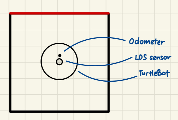
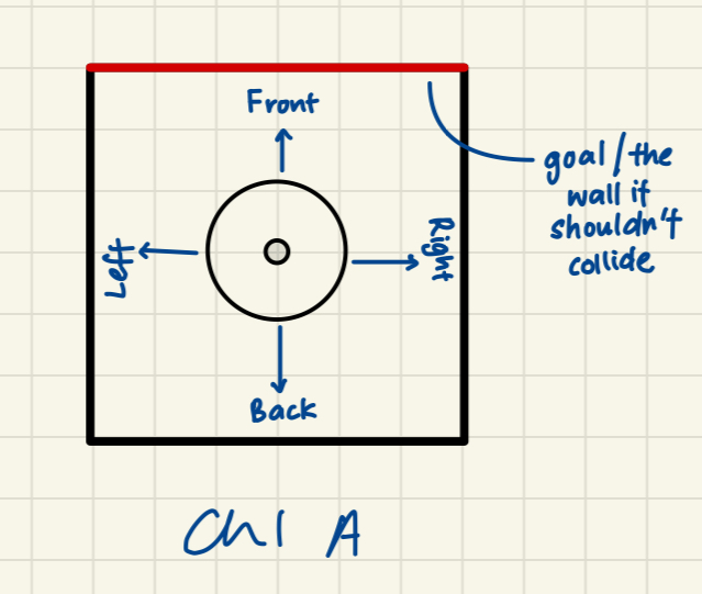
Figure 1: Initial objects in the scene (left) and goal description (right) for the first steps.

Velocity Control

Building upon the foundation laid previously, we choose the 1 x 1 meter maze setting. The principal task in this challenge was to navigate the robot to a wall without collision. Furthermore, additional requirements necessitated the implementation of smooth acceleration and deceleration to facilitate seamless motion control.

We implemented the subscription to the LIDAR sensors data and the publisher to change the Velocity of the robot's wheels. Using this, it was simple to write a program that checked the distance to the front wall and calculated its speed based on this distance. If the distance was greater than 0.3m, it would accelerate and then decelerate as soon as it crossed that boundary. We made sure to include a minimum speed that was reasonable, so that the robot would eventually reach its destination and not slow down to almost 0 before it got there. I also made sure to include a safety distance to the wall, as the LIDAR is around 8cm back from the front of the robot, and if you don't account for this, the robot will never stop, since the LIDAR never returns a distance of 0.

Objectives

• Use the Laser Distance Sensor (LDS) to measure the distance between the robot and obstacles in its path.
• Implement proportional control for velocity adjustment based on the distance to the obstacle.
• Ensure the robot decelerates smoothly as it approaches the wall and comes to a complete stop at a safe distance.
• Handle sensor noise effectively to maintain robust and accurate performance.

Approach

We utilized ROS2 nodes to process sensor data and control the robot's motion. The robot was required to adjust its speed dynamically based on the distance to the obstacle, ensuring smooth acceleration and deceleration.

1. Laser Distance Sensor (LDS) Data Processing

The LDS provides an array of distances in a 360° sweep around the robot. For this challenge, only the distance directly in front of the robot was relevant. To handle sensor noise, multiple readings were averaged using a moving window technique, ensuring stable and accurate measurements.

def scan_callback(self, msg):
    # Extract front distance
    front_distance = msg.ranges[0]

    # Filter noisy data
    if front_distance == float('inf') or front_distance <= 0:
        self.get_logger().warning("Invalid sensor reading!")
        return

    # Add to moving window
    self.distance_window.append(front_distance)
    if len(self.distance_window) > self.window_size:
        self.distance_window.pop(0)

    # Calculate average distance
    avg_distance = sum(self.distance_window) / len(self.distance_window)
    self.get_logger().info(f"Averaged Distance: {avg_distance}")

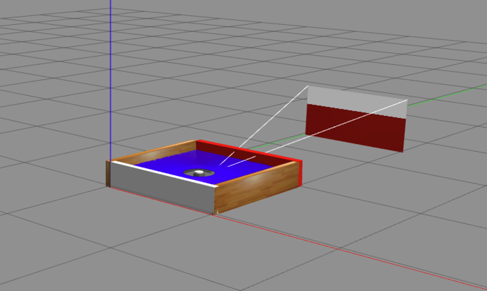
Figure 1: Screenshot from Gazebo simulator.

2. Proportional Velocity Control

A proportional controller was implemented to adjust the robot's linear velocity based on the distance to the wall. The velocity was calculated using the formula:

Velocity = Proportional_Gain × (Distance - Safety_Distance)

The proportional gain ensured that the velocity was directly proportional to the distance, resulting in smooth deceleration as the robot approached the wall. A minimum velocity threshold was set to prevent the robot from stalling prematurely.

def calculate_velocity(self, distance, safety_distance=0.3):
    # Define proportional gain
    proportional_gain = 0.5
    # Calculate velocity
    velocity = proportional_gain * (distance - safety_distance)
    # Enforce minimum velocity for smooth motion
    return max(0.05, velocity) if distance > safety_distance else 0

3. Integration with ROS2

The proportional velocity control logic was integrated into a ROS2 node, which subscribed to the /scan topic for LDS data and published commands to the /cmd_vel topic for velocity control. The following flow illustrates the interaction between components:

Figure 2: ROS2 node interaction for velocity control and sensor data processing.

Challenge 2: Precise Rotation

Building upon the accomplishments of Challenge 1, Challenge 2 focused on achieving precise rotational alignment. The principal objective was to enable the TurtleBot to perform an exact 90-degree counterclockwise rotation within the established maze environment. This challenge introduced the complexity of combining Laser Distance Sensor (LDS) data and odometry to ensure accuracy.

Challenge 2 benefited from leveraging a foundational template that provided basic ROS2 subscriptions for sensor data and publishers for wheel velocities. Using these, a robust algorithm was developed to calculate rotational errors and control the robot's angular velocity. The process ensured that the TurtleBot aligned precisely with the desired orientation without overshooting or undershooting.

Objectives

• Accurately rotate the TurtleBot by 90 degrees counterclockwise.
• Utilize LDS data and odometry for precise alignment and error correction.
• Implement smooth rotational control to prevent abrupt motions.
• Handle sensor noise effectively to ensure robust performance.

Approach

Challenge 2 required a creative combination of geometric transformations and control logic to achieve precise rotation. Data from the LDS was carefully calibrated to reflect the robot's central frame of reference, while odometry tracked incremental rotational changes.

1. LDS Data Transformation

The LDS data, originally captured in the sensor's frame, was transformed into the robot's central frame to account for the offset of the LDS. This transformation ensured accurate and reliable distance measurements relative to the axis of rotation.

def lds_to_robot(self, point):
    x_lds = point[0] * math.cos(point[1])
    y_lds = point[0] * math.sin(point[1])
    x_robot = x_lds - 0.065  # LDS offset of 6.5 cm
    y_robot = y_lds
    distance_robot = math.sqrt(x_robot**2 + y_robot**2)
    angle_robot = math.atan2(y_robot, x_robot)
    return distance_robot, angle_robot

2. Rotation Error Calculation

The rotational error was determined by comparing the current orientation with the target orientation. This calculation leveraged odometry data to track incremental rotational changes and normalize the error within a manageable range.

def calculate_rotation_error(self, target_angle, current_angle):
    error = target_angle - current_angle
    return (error + math.pi) % (2 * math.pi) - math.pi  # Normalize between -π and π

3. Proportional Rotation Control

A proportional controller was implemented to dynamically adjust angular velocity based on the rotation error. This approach ensured that the robot decelerated smoothly as it approached the target angle, resulting in precise alignment.

def calculate_angular_velocity(self, rotation_error):
    proportional_gain = 1.0
    angular_velocity = proportional_gain * rotation_error
    return max(-1.0, min(1.0, angular_velocity))  # Clamp angular velocity

4. Integration with ROS2

The rotational control logic was encapsulated in a ROS2 node that subscribed to odometry data and published angular velocity commands to the TurtleBot. This node continuously monitored rotation error and dynamically adjusted angular velocity for precise control.

Challenge 3: Sequential Movement

Building upon the previous challenges, Challenge 3 demonstrated the TurtleBot's ability to execute a sequence of precise movements and rotations. The task required the robot to move forward 15 cm, perform an exact 90-degree rotation, and move forward another 15 cm, all while maintaining high accuracy and smooth transitions.

The implementation relied on a state machine to manage sequential actions, leveraging odometry for precise tracking and control. Each action was executed with a clear target and carefully calibrated motion control, ensuring robust and repeatable performance.

Objectives

• Program the TurtleBot to move forward exactly 15 cm, rotate 90 degrees, and move forward another 15 cm.
• Utilize odometry data for accurate tracking of position and orientation.
• Implement a state machine to manage and coordinate the sequence of movements.
• Ensure smooth transitions between movements to maintain stability.

Approach

This challenge required the integration of precise motion tracking, rotational control, and sequential logic. A modular approach was adopted to separate each movement phase, enabling efficient debugging and future adaptability.

1. State Machine Design

A state machine was implemented to orchestrate the movement sequence. The robot transitioned between the following states:

• MOVE_FORWARD: Move forward 15 cm while tracking distance using odometry.
• ROTATE: Perform a 90-degree clockwise rotation with odometry-based angle tracking.
• MOVE_FORWARD_2: Move forward another 15 cm after completing the rotation.

2. Odometry for Accurate Tracking

Odometry provided real-time feedback on the robot's position and orientation. By continuously monitoring x, y, and yaw values, the robot calculated distances traveled and angles rotated with precision.

def calculate_distance(self, start_pose, current_pose):
    dx = current_pose.x - start_pose.x
    dy = current_pose.y - start_pose.y
    return math.sqrt(dx**2 + dy**2)

3. Smooth Motion Control

Proportional control algorithms were applied to both linear and angular velocities to ensure smooth motion. The robot gradually reduced velocity as it approached the target position or orientation, preventing abrupt stops.

def control_velocity(self, error, max_speed):
    proportional_gain = 0.5
    velocity = proportional_gain * error
    return max(-max_speed, min(max_speed, velocity))  # Clamp velocity

4. Integration with ROS2

The control logic was implemented in a ROS2 node that subscribed to odometry data and published velocity commands. The state machine logic ensured modularity, with each state triggering specific commands to achieve its respective goal.

Challenge 4: Maze Navigation

Here we marked a significant progression in the TurtleBot's capabilities, involving navigation through increasingly complex mazes. First, the robot navigated a 2x2 maze, and then we extended this to a 3x3 maze. These challenges required advanced techniques in mapping, pathfinding, and odometry correction to ensure accurate and efficient traversal of the maze environments.

Objectives

• Navigate a 2x2 and a 3x3 maze from the bottom-left corner to the top-right corner.
• Develop a dynamic wall detection system using the Laser Distance Sensor (LDS).
• Implement the A* search algorithm for optimal pathfinding within the maze.
• Correct odometry drift for precise positioning and navigation.

Approach

The challenges combined perception, planning, and control into a cohesive navigation framework. The robot dynamically updated its internal map, calculated optimal paths using A*, and executed precise movements to traverse the maze step-by-step.

1. Wall Detection and Mapping

The LDS was used to detect and map walls around the robot dynamically. Each cell in the maze was represented as a grid, and obstacles were marked based on sensor readings. This mapping approach included:

• World Transformation: Converting LDS readings into world coordinates relative to the robot.
• Grid Representation: Mapping world coordinates to grid cells for easy pathfinding.
• Obstacle Marking: Dynamically identifying and marking walls in the grid.

In this task, the aim is to navigate the robot from the lower-left extremity to the upper-right extremity of a maze by leveraging data from both the odometer and the laser distance sensor. The methodology commences with the initialization of the maze dimensions, setting the starting point and the target destination within the grid.

The `world_size` parameter delineates the overall dimensions of the maze in meters, while the `cell_size` defines the spatial extent of each individual cell within this maze in meters. The matrix `self.grid` is initially populated with zeros, symbolizing an absence of obstacle knowledge at the outset, with the robot being aware solely of the maze's dimensions.

def map_walls(self, lds_readings):
    for angle, distance in lds_readings.items():
        if distance < self.max_sensor_range:
            x_world = self.robot_x + distance * math.cos(angle)
            y_world = self.robot_y + distance * math.sin(angle)
            grid_x, grid_y = self.world_to_grid(x_world, y_world)
            self.grid[grid_x][grid_y] = 1  # Mark as occupied

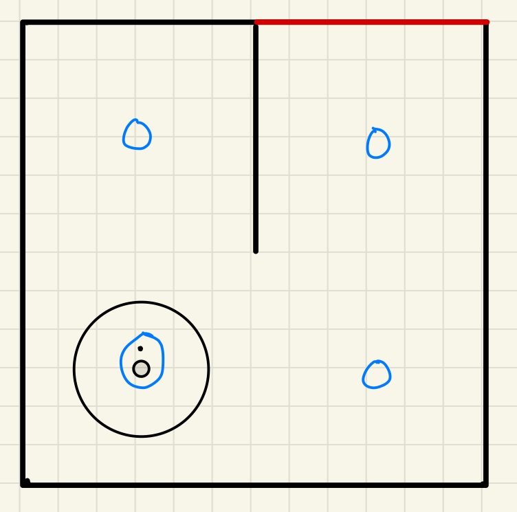
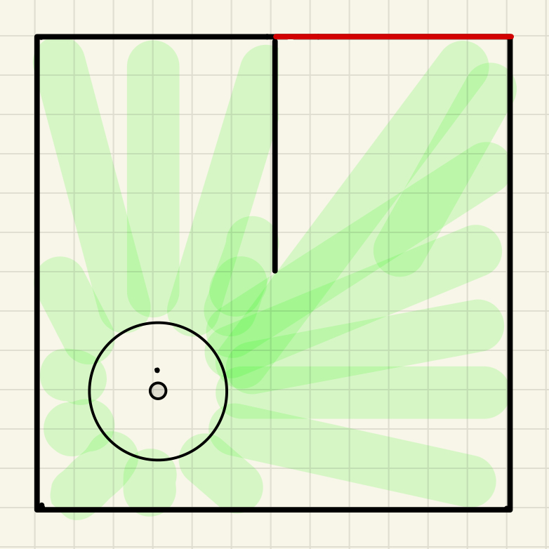
Figure 2: initialised grids in zeros (left) and the range of the LDS sensor while the robot is in its initial position (right) of a maze world in the form of 2 x 2 meters.

With this setup, the robot gains awareness of its spatial context within the maze and its ultimate objective. Utilizing the laser distance sensor, the robot identifies wall locations, translating these detections from the LDS frame to the robot's frame, then to the world frame, and ultimately into grid coordinates. These transformations facilitate the subsequent updating of the maze's grid map, marking cells as occupied based on the sensor data.

As the robot detects the walls, it will be consider as "1". Upon refreshing the grid map with obstacle information, the robot employs the A* search algorithm to ascertain a viable path to the target. This algorithm is designed to identify the most efficient route, avoiding occupied cells based on the updated grid information. The presence of an obstacle in a cell disqualifies it from being part of the calculated path. After the process from above then it will mark the grids that is occupied or blocked as 1 in the grid matrix.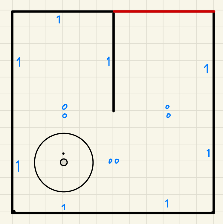

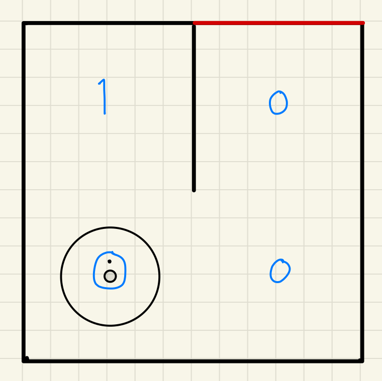
Figure 3: detecting walls in various directions (left) and identifying blocked paths in the grid (right) of a maze world in the form of 2 x 2 meters.

Upon identifying a viable pathway, the robot engages its control systems to traverse the established route. This process involves utilizing data from the Laser Distance Sensor (LDS) to continuously ascertain the presence of any newly detected barriers, especially after reaching the end of the path but before arriving at the goal. Additionally, it employs odometric information to maintain awareness of its positional and orientational status. The implementation of this methodological approach is anticipated to facilitate the robot's successful navigation to the predetermined target location within the labyrinthine environment.

Voila! This image show how the robot should drive towards its end goal and stop: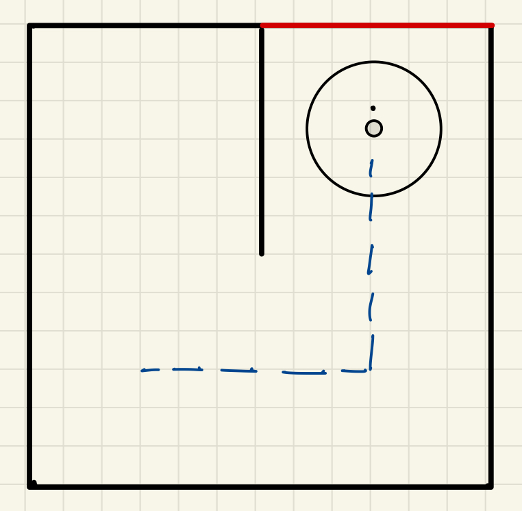

Figure 4: Predicted path in a maze world in the form of 2 x 2 meters.

The second strategy for this challenge involves utilizing odometer data for the robot to ascertain its position and orientation for navigation. Concurrently, data from the laser distance sensor will be employed to detect obstacles, such as walls.

Upon determining the distance between the robot and a wall that impedes its trajectory towards the goal, should the laser distance sensor register a distance less than 1.73 meters at an approximate angle of 30 degrees to the right, the robot will ascertain the presence of a wall. In such an instance, the robot will deduce that it must adopt the lower route, which entails rotating right, advancing straight, rotating left, and then proceeding straight towards its destination. Should the lower route be obstructed, the robot will then resort to the upper route, characterized by moving straight, executing a right rotation, and continuing in a straight line until it reaches its objective.

This approach will only work if the world is a 2 x 2 meters maze. It is a simpler approach to solve this challenge.

2. Wall Detection and Mapping for 3x3 maze

The figure below shows one of the 3 x 3 meters maze world with the robot finding it's path to the goal state. We use the same approach as before, as it is dynamic. The robot's LDS sensor is able to detect the wall and the range of the LDS sensor is noted in green spacing. The red marking shows the grid matrix values. The blue marking shows the where the walls are detected in each grid cell. At the end, it will drive and arrive at its goal.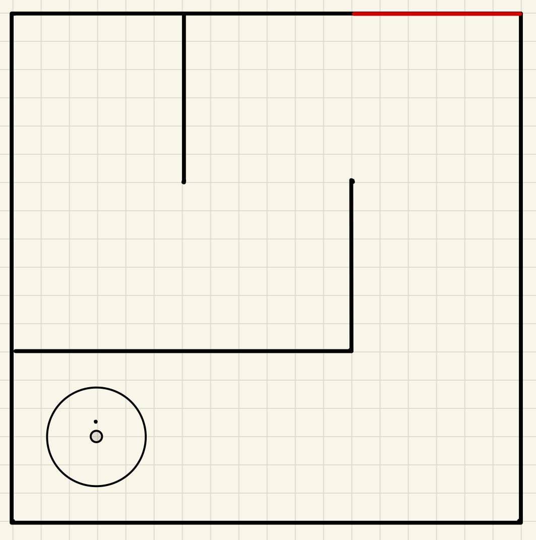

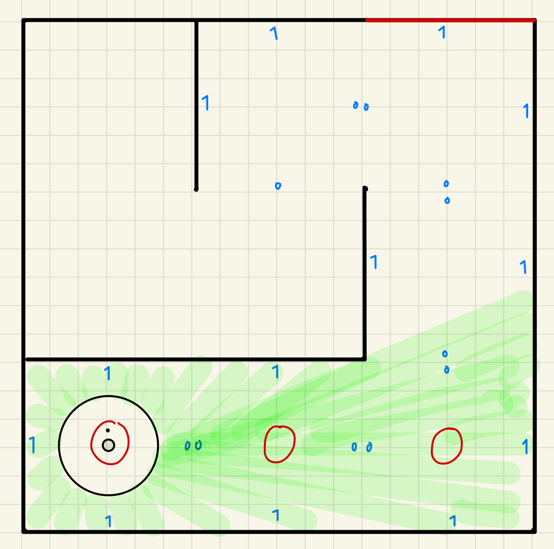
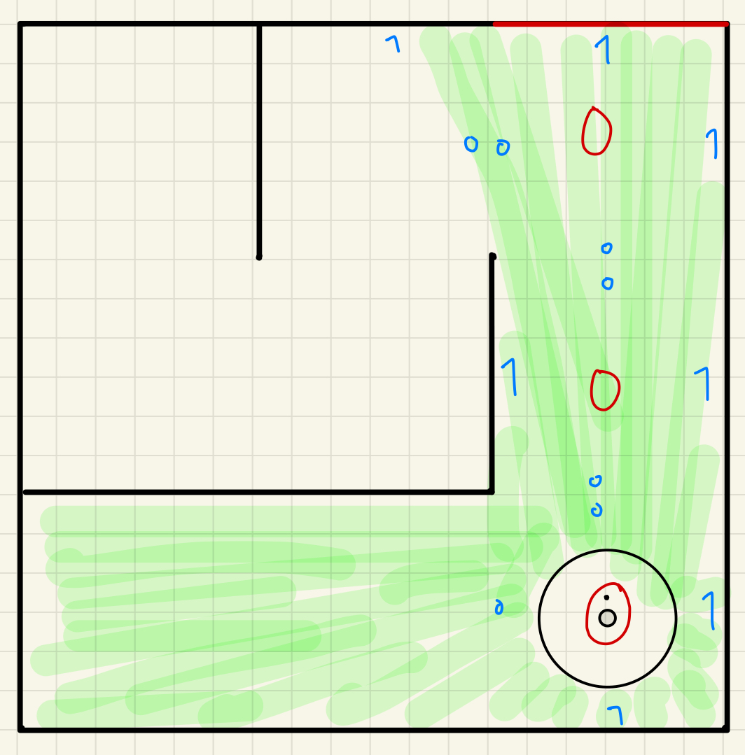
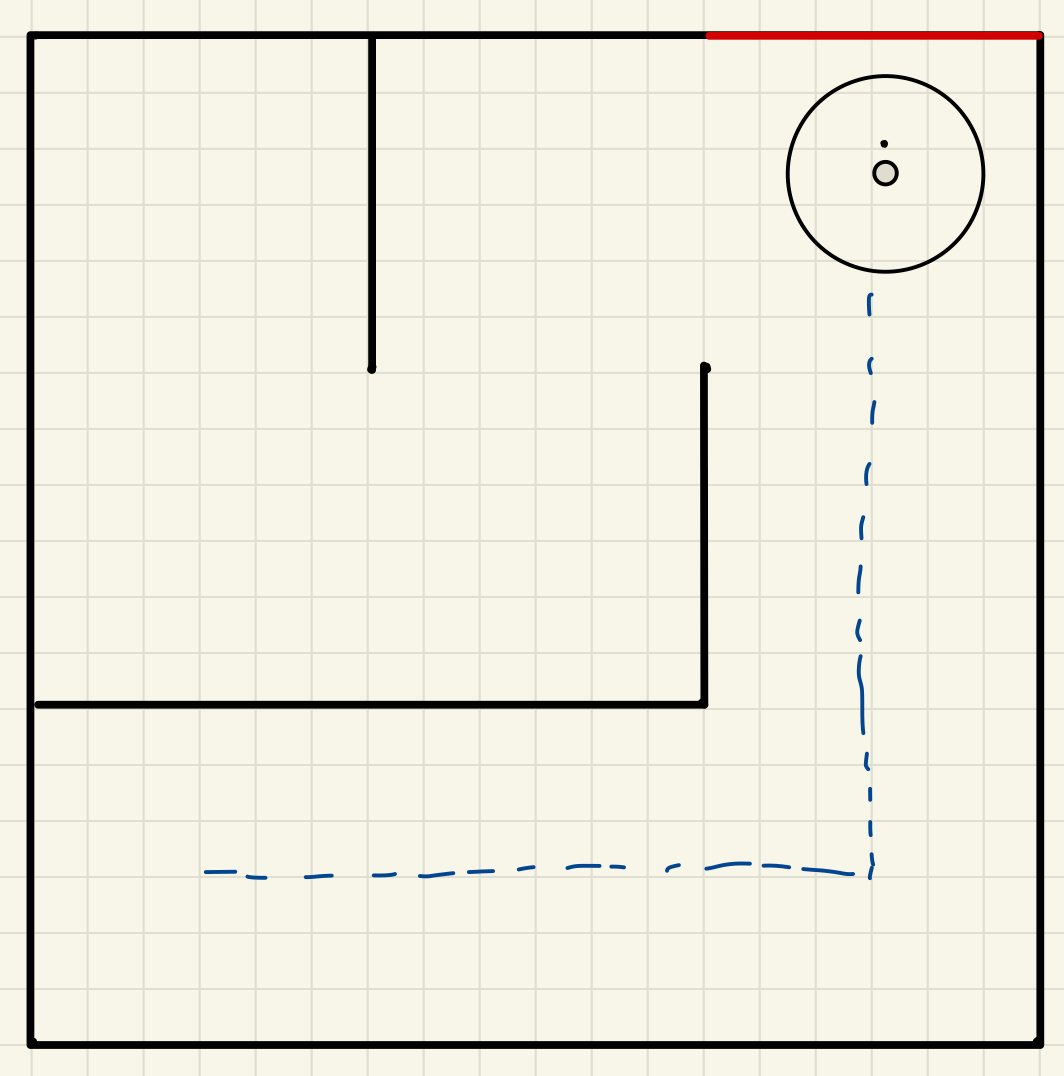
Figure 5: initial position (left), identifying blocked paths in the grid (center), and final trajectory (right) in the 3 x 3 meters maze.

3. Pathfinding with A* Algorithm

The A* search algorithm provided an optimal path to navigate from the starting position to the goal. The algorithm utilized a heuristic (Manhattan distance) to efficiently balance exploration and exploitation. The pathfinding process included:

• Open List: Prioritized nodes to explore based on cost.
• Closed List: Nodes that were already evaluated.
• Cost Calculation: Combining movement cost (g) and heuristic (h) to determine priority.

def a_star_search(self, start, goal):
    open_list = PriorityQueue()
    open_list.put((0, start))
    came_from = {}
    cost_so_far = {start: 0}

    while not open_list.empty():
        current = open_list.get()[1]

        if current == goal:
            break

        for neighbor in self.get_neighbors(current):
            new_cost = cost_so_far[current] + self.get_cost(current, neighbor)
            if neighbor not in cost_so_far or new_cost < cost_so_far[neighbor]:
                cost_so_far[neighbor] = new_cost
                priority = new_cost + self.heuristic(neighbor, goal)
                open_list.put((priority, neighbor))
                came_from[neighbor] = current
    return self.reconstruct_path(came_from, start, goal)

Figure 2: Visualization of A* search algorithm used to solve a maze.

3. Sequential Navigation and Correction

After computing the optimal path, the robot executed each step sequentially. Periodic corrections, such as wall alignment, ensured that odometry drift did not compromise navigation accuracy. Key components included:

• Wall Alignment: Correcting orientation by aligning LDS readings with detected walls.
• State Machine: Managing movement states like move forward, rotate, and correct drift.

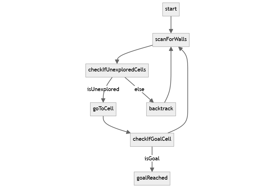
Figure 3: State machine for sequential navigation in a maze.